Monitoring with the TIG Stack

One day I'll implement Prometheus (a more free and open software) in place of InfluxDB but I haven't had the opportunity yet, so today we talk about the TIG stack:

• Telegraf records data about the state of a machine, and sends it to
• InfluxDB which stores the data as time-series data, to be read by
• Grafana which displays real-time graphs in a dashboard

Let's start with a dashboard screenshot:

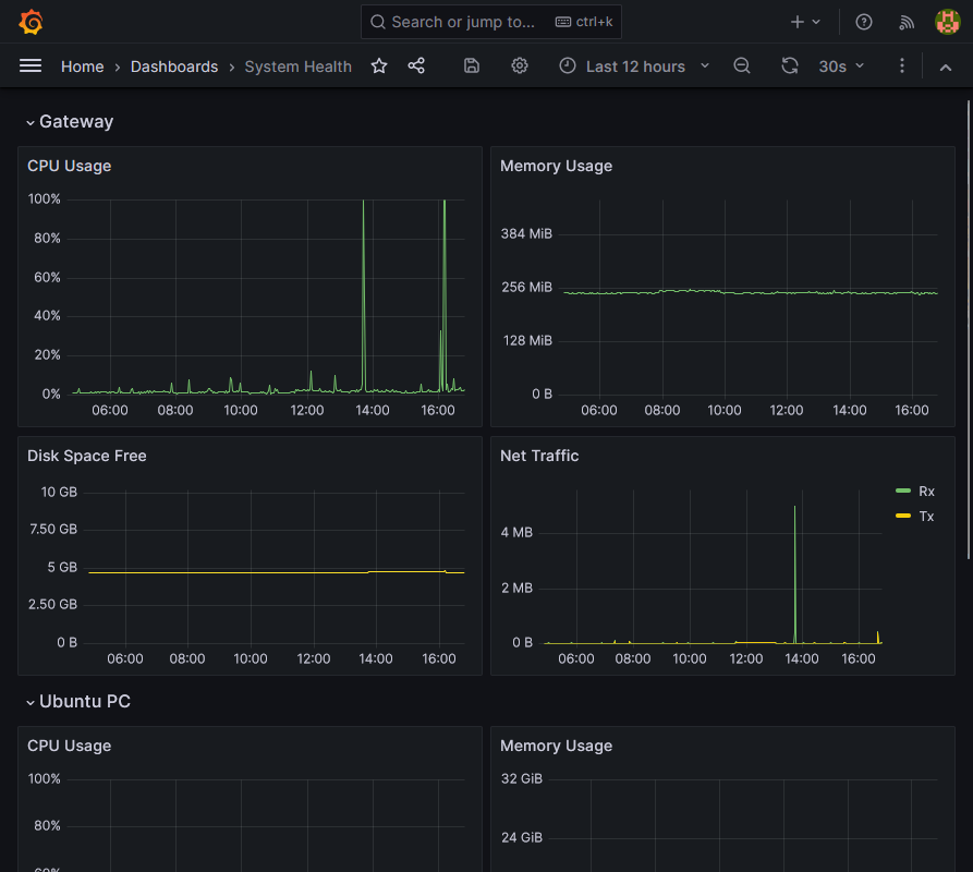
It never hurts to be able to have metrics for your various machines available at a glance, but there's so much more you can do than just imitate Task Manager. See this post and the followup for a great writeup.

Some software issues are just hardware or system issues in disguise, so it pays to have easy access to information about system health across an organisation. Whether you need to find a bottleneck or just check that all machines are running or have network connectivity, when the issue arises, you'll be glad you set this up.

Deploy It

Without further ado, some configs:

version: '2'

services:

  influxdb:
    image: influxdb:alpine
    restart: unless-stopped
    ports:
      - '12102:8086'
    volumes:
      - ./influxdb/data:/var/lib/influxdb2:rw
    environment:
      - DOCKER_INFLUXDB_INIT_MODE=setup
      - DOCKER_INFLUXDB_INIT_USERNAME=${INFLUXDB_USERNAME}
      - DOCKER_INFLUXDB_INIT_PASSWORD=${INFLUXDB_PASSWORD}
      - DOCKER_INFLUXDB_INIT_ORG=${INFLUXDB_DEFAULT_ORG}
      - DOCKER_INFLUXDB_INIT_BUCKET=${INFLUXDB_PRIMARY_BUCKET}
      - DOCKER_INFLUXDB_INIT_RETENTION=${INFLUXDB_PRIMARY_BUCKET_RETENTION}
      - DOCKER_INFLUXDB_INIT_ADMIN_TOKEN=${INFLUXDB_ADMIN_TOKEN}

  grafana:
    image: grafana/grafana:latest
    restart: unless-stopped
    ports:
      - '12101:3000'
    volumes:
      - ./grafana/data:/var/lib/grafana
      - ./grafana/provisioning/:/etc/grafana/provisioning
    depends_on:
      - influxdb
    environment:
      - GF_SECURITY_ADMIN_USER=${GRAFANA_USERNAME}
      - GF_SECURITY_ADMIN_PASSWORD=${GRAFANA_PASSWORD}

INFLUXDB_USERNAME=admin
INFLUXDB_PASSWORD=correct-horse-battery-staple
INFLUXDB_DEFAULT_ORG=lchapman.dev
INFLUXDB_PRIMARY_BUCKET=weekly
INFLUXDB_PRIMARY_BUCKET_RETENTION=7d
INFLUXDB_ADMIN_TOKEN=right-brumby-capacitor-fastener

GRAFANA_USERNAME=admin
GRAFANA_PASSWORD=running-out-of-ideas

...

# Grafana
http://grafana.lchapman.dev {
        reverse_proxy localhost:12101
}

# Influx
http://influx.lchapman.dev {
        reverse_proxy localhost:12102
}

...

Some notes:

1. See my post about Caddy for more details about the Caddyfile.
2. I use the default org for my personal infrastructure, then any specific infrastructure (for a client, for example) will use a separate org (i.e. client1.lchapman.dev).
3. The choice of 7 days of retention is arbitrary, choose a time interval that suits your needs.
4. The InfluxDB volume needs to point to the influxdb2 folder. The compose file I worked from originally had been adapted from InfluxDB v1 (where the folder was just influxdb) and therefore my first couple of trial runs had no persistence.

So that's the database and the dashboard set up in containers, but where does the data come from? Initially I had Telegraf running in the compose stack but the system stats that were coming from it were related to the container rather than the system, so it becomes one of the rare softwares I install using more traditional means. See here for details. After that, deploy your config and off you go.

# For InfluxDB OSS 2:
[[outputs.influxdb_v2]]
  urls = ["https://influx.lchapman.dev"]
  token = "your-token-here-but-don't-forget-to-make-it-first"
  organization = "lchapman.dev"
  bucket = "weekly"

[agent]
  interval = "10s"
  hostname = "gateway"

# Inputs

[[inputs.cpu]]
  percpu = true
  totalcpu = true
  collect_cpu_time = false
  report_active = false
[[inputs.disk]]
  ignore_fs = ["tmpfs", "devtmpfs", "devfs", "iso9660", "overlay", "aufs", "squashfs"]
[[inputs.diskio]]
[[inputs.mem]]
[[inputs.net]]
  interfaces = ["eth*", "tun0", "lo"]
[[inputs.processes]]
[[inputs.swap]]
[[inputs.system]]

More notes:

1. The URL represents the route to my InfluxDB. If you're running multiple databases you can specify multiple destinations. Neat.
2. The token doesn't exist yet. Go to Influx > Load Data > API Tokens > Generate API Token (Custom API Token). Name it something descriptive like weekly_Telegraf_gateway, give it write access to the weekly bucket and click Generate.
3. The outputs.influxdb_v2 section will be consistent across all of your machines, but the agent section will not. Set the hostname per machine.
4. The inputs section here is populated with a template I found useful, but do check out the Telegraf docs to get the data you care about. There's a whole ecosystem of plugins. Seriously, check it out.

Display It

We have a database that is being populated: great! Let's see it then. InfluxDBv2 uses its own language to query data called Flux. Flux lang is flexible and readable and while not everybody is happy that it replaced the SQL-like language used in InfluxDBv1, it's fine. Having to learn yet another language is fine. It's fine.

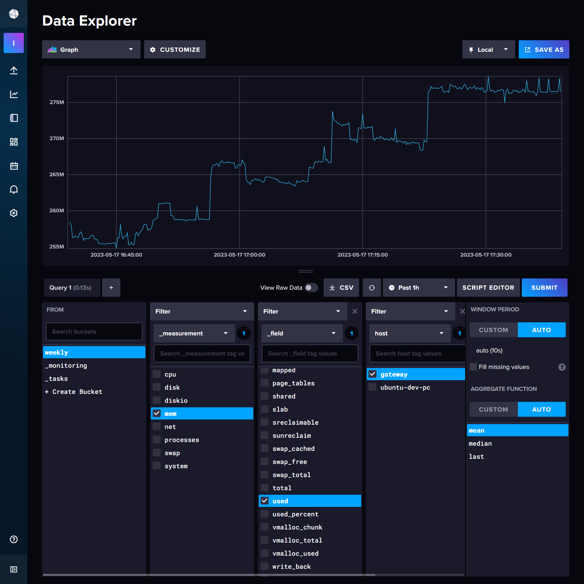
Use the Data Explorer within your Influx web interface to start crafting your queries, then click Script Editor to access the actual Flux query.

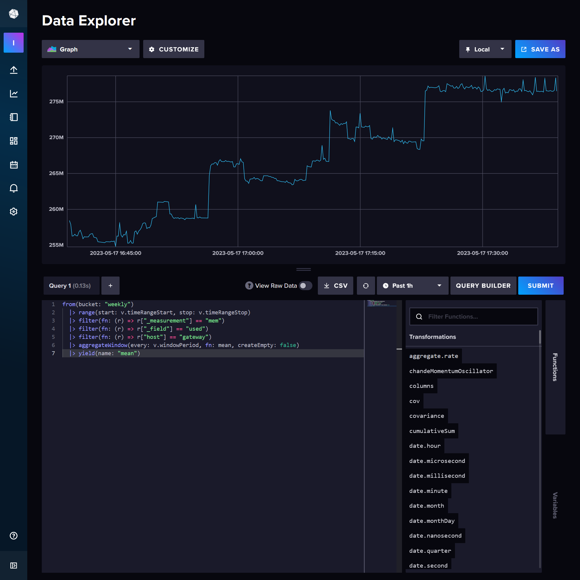
from(bucket: "weekly")
  |> range(start: v.timeRangeStart, stop: v.timeRangeStop)
  |> filter(fn: (r) => r["_measurement"] == "mem")
  |> filter(fn: (r) => r["_field"] == "used")
  |> filter(fn: (r) => r["host"] == "gateway")
  |> aggregateWindow(every: v.windowPeriod, fn: mean, createEmpty: false)
  |> yield(name: "mean")

It's all pretty easy to follow, except maybe the v variable which is supplied by the viewer, in this case the Data Explorer but later it will be Grafana. The highest level of data organisation is in a "measurement" which contains some "field". Past that there are tags, such as the host tag here which is set by Telegraf as per our config.

The aggregateWindow function is worth explaining. Without it, the request could return an arbitrarily large number of datapoints, and while I do love high levels of precision, there's a tradeoff to be made regarding the load placed on the database, especially if your dashboard is set to update every 10 seconds. The value passed to every could be a constant, like 1m (1 minute), or it can be dynamic, like v.windowPeriod: a 24 hour window produces 2m period, 7 days is 15m, 2 hours is 10s and anything less is actually doing nothing because my data collection interval is 10 seconds anyway. Set createEmpty to true if your machine ever powers off; there's not much reason to leave it false regardless. For my graphs of CPU usage I set the aggregate function to max rather than mean because I'm looking for bottlenecks and mean hides them.

A new Grafana instance may require you to head to the Connections menu and configure the InfluxDB connection. Use the Flux query language rather than InfluxQL, it's the one in active development. I found that the URL field works fine as either of http://influxdb:8086 or https://influx.lchapman.dev/, with the former being preferable because traffic need not exit the container stack in this case. Turn off the basic auth toggle. Set the organization and default bucket as per your environmental variables. Min time interval of 10s is correct here because that's my minimum data write period.

The token I supply to Grafana doesn't exist yet either. I create a read-only token for the weekly bucket called weekly_Grafana. Paste it in, click save & test and you should see a green tick and the message "datasource is working. 1 buckets found".

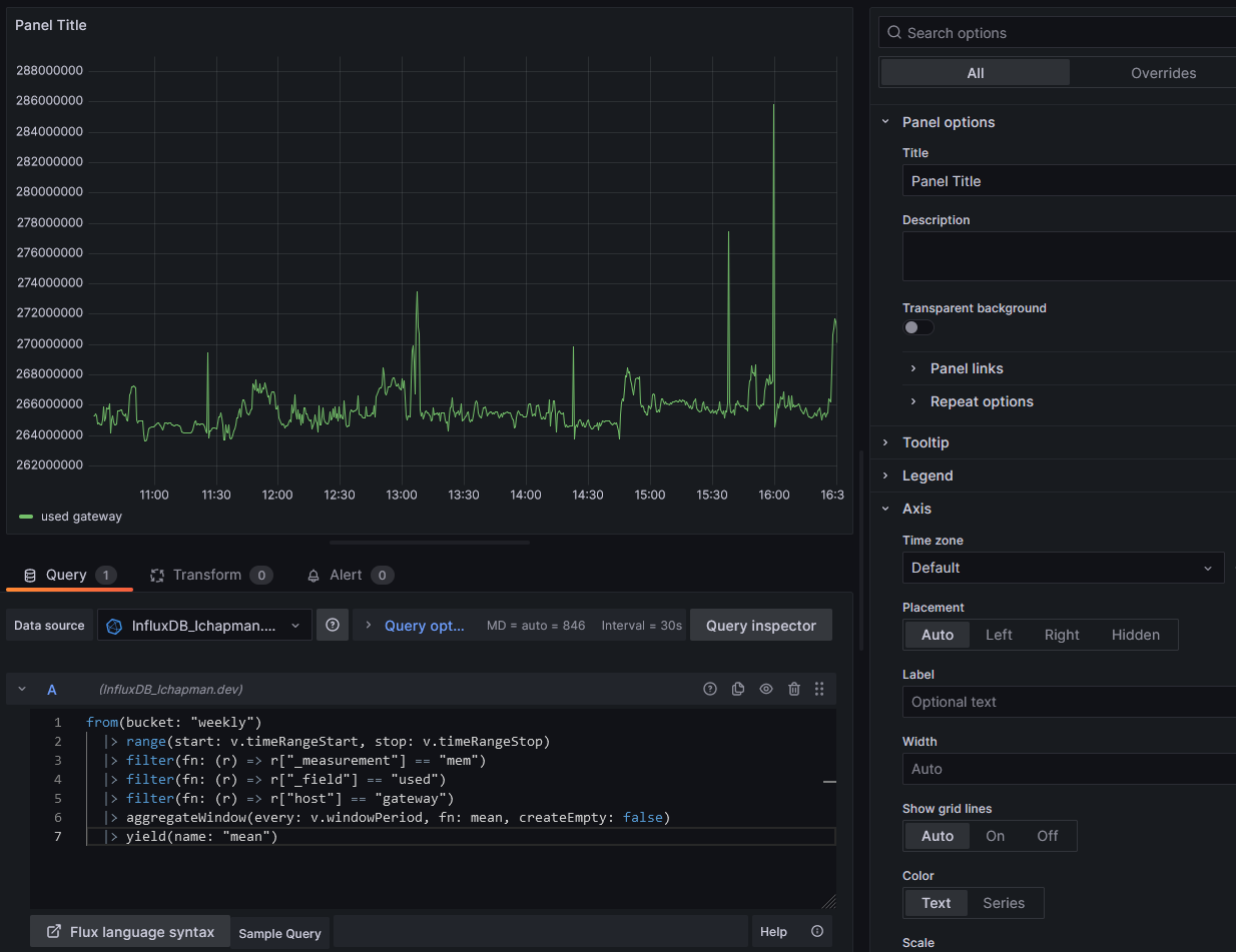
Now you'll want to go to Dashboards > New Dashboard > Add vizualization, paste the query from Influx into the A query, then click somewhere outside the query textbox. Grafana will see your changes and load the data. If it looks good, click Save. In my case, I'll want to fiddle with the options a bit. Set the unit to bytes (SI) in Standard Options and while I'm there I'll set a min and max. A proper title helps too.

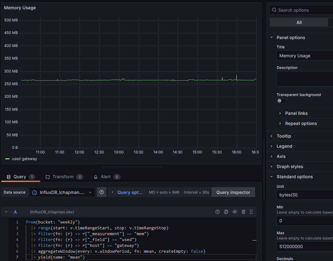
One last lesson before I wrap this up: computed series names. If you're doing a per-core CPU graph, you'll immediately see an issue:

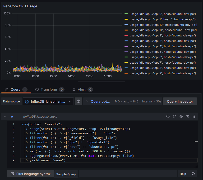
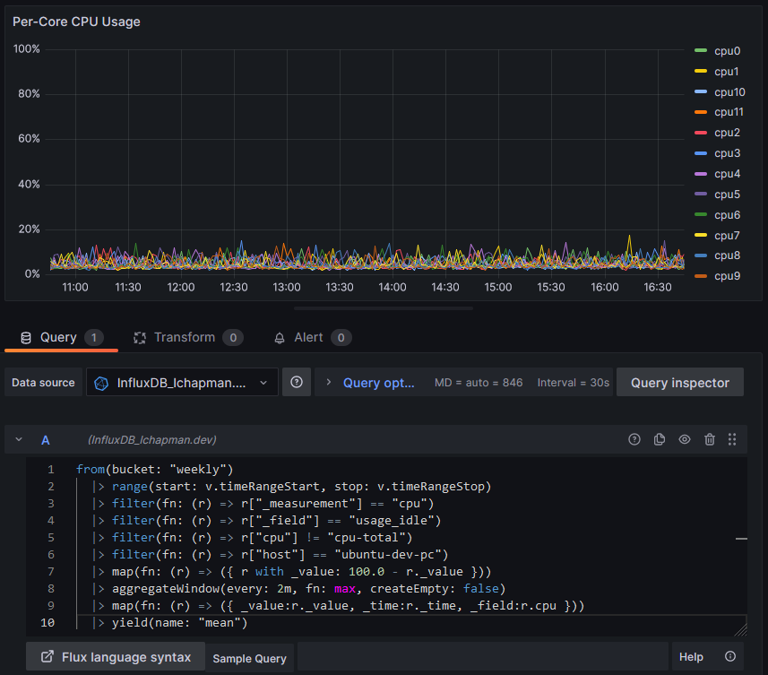
Note the map function to apply a transform to every data point, converting a measurement of core idleness to core busy-ness. Also note the legend being awful due to series names being just daft. I suppose it's a sensible default behaviour but it falls apart in this particular use case. Here's our silver bullet:

  |> map(fn: (r) => ({ _value:r._value, _time:r._time, _field:r.cpu }))

Time and value are passed through but the field name is overwritten by just the value of the cpu tag. Handy! I suppose I could write a function to strip the "cpu" part from "cpu7" but... I'm not going to. The result:

The eagle-eyed amongst you will notice a lack of optimisation: why not move the first map function after the aggregateWindow, reducing the number of rows the map operates on? Doing so reduces the query time from 500ms to 350ms. Moving the minus operation into the second map and removing the first altogether brings it down to 280ms, for a total reduction of processing time of 45% - not bad. My sample sizes for this data were ~2, hardly rigorous, but there really is a measurable change. Combining the filter calls from 4 to 1 (a series of and statements) however does not elicit any performance gains worth noting, and reduces readability to miserable lows.

There's plenty more I'll learn about Flux-lang as I go, but for now, I don't mind it. It seems to have the tools I need. I'll try Prometheus one day, but not today.